Pseudorandom numbers and linear congruential genrators

Exploring pseudorandom number generators.

Pseudorandom number generators (PRNGs) are algorithms for generating sequences of numbers, that appear — according to some chosen special qualities — to have been chosen at random.

People devising simulations and other software, have for a long time faced a choice when trying to acquire random numbers: Whether to rely on a physical process, or to use a mathematical process.

A physical process, while random may have unknown and undesired properties. A mathematical one on the the other hand is not truly random at all, but its properties may be better known.

Any one who considers arithmetical
methods of producing random digits
is, of course, in a state of sin.

John Von Neumann, 1951.

The above famous quote is easy to misinterpret. It’s less known, that the quote continues¹ by

[It is] a problem that we suspect of being solvable by some rigorously defined sequence.

Von Neumann needed randomness for Monte Carlo simulation.

Alas, the need for random numbers grew in the first half of the 20’th century. In 1955 the RAND corporation even published a 400 page book titled A Million Random Digits with 100,000 Normal Deviates.

Since then, many algorithms have been devised for generating pseudorandom numbers.

The equidistribution theorem

The equidistribution theorem states that, for an irrational constant $c$, the sequence

$$\left\{ 0, c, 2c, 3c, 4c,\cdots\right\}\bmod 1$$

is uniformly distributed.

Shifting the sequence with a constant $s_{0}$ retains this property. In other words, for a non negative integer, $n \in \mathbb{N}_0$, the sequence:

$$\tag{1} \label{eq:1} \boxed{ s_{n}=\left(n\thinspace c + \thinspace s_{0} \right)\bmod 1 }$$

produces uniformly distributed values in the interval $\left[0,1\right)$.

Note, that since

$$\begin{aligned} s_{n}&=\left(n\thinspace c + s_{0} \right) &\bmod 1 \\ s_{n+1}&=\left((n+1)\thinspace c + s_{0} \right) &\bmod 1 \\ \end{aligned}$$

we can rewrite the recurrence as:

$$s_{n+1}=\left((n \thinspace c + s_{0}) + c \right)\bmod 1$$

Substituting $s_n$ for $\left(n \thinspace c + s_{0} \right) \bmod 1$ gives us a recurrence relation:

$$\tag{2} \label{eq:2} s_{n+1}=\left(s_{n} + c \right)\bmod 1$$

This is the starting point of our PRNG.

A geometric interpretation

An interesting geometric interpretation for our sequence is presented in the book Fourier Analysis: An Introduction²:

Suppose that the sides of a square are reflecting mirrors and that a ray of light leaves a point inside the square. What kind of path will the light trace out?

…

the reader may observe that the path will be either closed and periodic, or it will be dense in the square. The first of these situations will happen if and only if the slope $\gamma$ of the initial direction of the light (determined with respect to one of the sides of the square) is rational.

To adapt the question to our notation, replace $\gamma$ with $c$ and consider $s_{n} \in \mathbb{R}^2$.

Here’s an Python implementation of simulating a ray bouncing in a square:

import matplotlib.pyplot as plt
import numpy as np
from numpy import array as vec2
from numpy.typing import NDArray as Vec2
from matplotlib.figure import Figure, Axes
from math import sqrt

EPSILON = np.finfo(np.float64).eps
SIZE = 10


def is_zero(a: np.float64) -> bool:
    return np.abs(a) < EPSILON * 2


def check_intersection(p: Vec2, step: Vec2, v: Vec2, s=10) -> tuple[np.number, Vec2, Vec2] | None:
    """Check intersection between a vector (step) with origin at point (p),
    and a square with a side of length (s)."""
    planes = (
        # tuples of [point on plane, normal, label]
        (vec2([0, s]), vec2([0, -1]), "top"),
        (vec2([s, 0]), vec2([-1, 0]), "right"),
        (vec2([s, 0]), vec2([0, 1]), "bottom"),
        (vec2([0, s]), vec2([1, 0]), "left"),
    )
    result = None
    for plane, normal, _ in planes:
        # disregard impossible hits along normal or with zero step
        if np.all(is_zero(step)) or step.dot(normal) == 0:
            continue

        # length along v
        l = (plane - p).dot(normal) / step.dot(normal)

        # disregard behind or far away
        if l < 0 or l > 1:
            continue

        # disregard hit on edge if facing inwards
        if is_zero(l) and v.dot(normal) > 0:
            continue

        # store closest hit
        if result is None or result[0] > l:
            p_hit = p + l * step
            result = l, p_hit, normal

    return result


def handle_intersection(l: np.number, p_hit: Vec2, n: Vec2, step: Vec2, v: Vec2):
    """Handle intersection at point (p_hit) at speed (v) and distance (step * l)
    with normal (n)"""
    # calculate remaining step from reflected penetation
    penetration = (1 - l) * v
    step = penetration - 2 * penetration.dot(n) * n

    # reflect velocity along normal
    v = v - 2 * v.dot(n) * n

    return p_hit, step, v


def calculate(p: Vec2, v: Vec2, steps: int, size: int) -> tuple[Vec2, Vec2]:
    """Calculate sequence of points for a ray from point (p) with velocity (v)
    bouncing in a square with side of length (size)"""
    points = [p]
    ray = [p]
    for _ in range(steps - 1):
        step = v
        while intersection := check_intersection(p, step, v, size):
            l, p_hit, n = intersection
            p, step, v = handle_intersection(l, p_hit, n, step, v)
            ray.append(p_hit)

        p = p + step

        points.append(p)
        ray.append(p)

        is_outside = p[0] < 0 or p[0] > size or p[1] < 0 or p[1] > size
        if is_outside:
            raise ArithmeticError("error due to numeric precision")

    return points, ray


if __name__ == "__main__":
    fig, ax = plt.subplots(1, 3, figsize=(8, 6), sharey=True, constrained_layout=True)
    plt.setp(ax, xlim=[0, SIZE], ylim=[0, SIZE], box_aspect=1)

    # starting point (p), velocity (c)
    p = vec2((3.5, 7.5))
    c = vec2((1.4, 1))

    plots = (
        # steps, velocity, fig. axis
        ( 20, c, ax[0]),
        (100, c, ax[1]),
        (400, c, ax[2]),
    )

    for steps, v, ax in plots:
        points, ray = calculate(p, v, steps, SIZE)

        ax.set(title=f"{steps} steps")
        ax.get_xaxis().set_visible(False)
        ax.get_yaxis().set_visible(False)

        ax.annotate("$P$", (p[0], p[1]), ha="right", va="baseline", fontsize=18)
        ax.scatter(*np.array(points).T, color="black")
        ax.plot(*np.array(ray).T, linewidth=1, color="black", clip_on=False)

    fig.suptitle("Bouncing ray\nwith velocity $c=(\\sqrt{2},1)$", fontsize=16, y=0.9)
    fig.savefig("reflections.png", bbox_inches="tight", pad_inches=0, dpi=300)
    plt.show()

In the above listing, we have defined the square to have sides of length 10. Each iteration, a light ray is advanced by its velocity $c$, and a sample point is recorded. By running the simulation with a rational velocity, we get figure figure 1.

Figure 1: Simulated reflections with c = (1.4, 1).

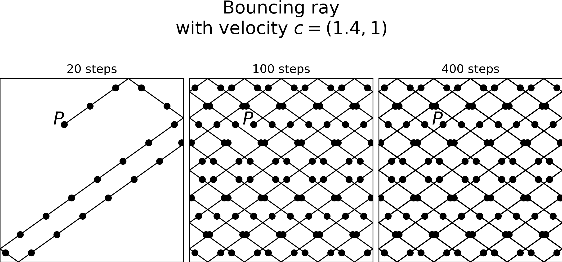
The figure shows an emerging grid pattern. The path of the bouncing ray is closed and has a period of 101 iterations.

What is of interest to us is the distribution of sample points along the x-axis. It’s evident, that the sequence won’t suffice as random enough.

When we change the velocity to an irrational constant, such as c = vec2((sqrt(2), 1)), we get figure figure 2.

Figure 2: Simulated reflections with c = (sqrt(2), 1).

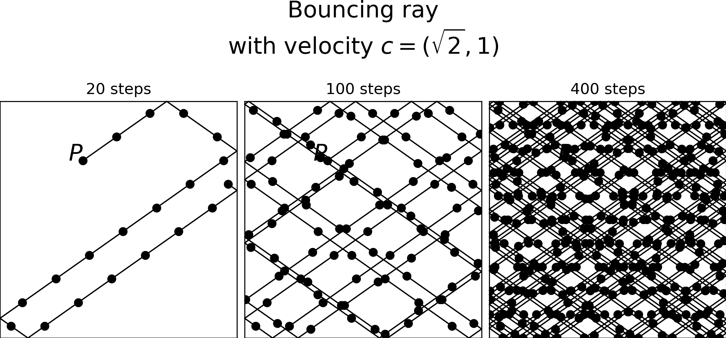
This time, the bouncing ray won’t fall into a recurring pattern. The produced sequence seems like a much better in terms of how random it appears visually. This is due to the theoretically infinite period, as predicted by the equidistribution theorem.

I say theoretically, because there’s a catch.

The catch

For the sequence to be usable, the calculations have to be performed with infinite-precision real numbers ³. In practice, evaluating a long sequence on the computers we have today will inevitably face floating-point errors. This means that the properties of our sequence break down, when $n$ is large.

To work around this, we’ll need to alter our sequence so that we can implement it on computers with limited precision.

Equation $\eqref{2}$ is a special case of a linear congruential generator (LCG). Using LCG’s for pseudorandom number generation dates back to the 1950’s⁴. Their quality is nowadays regarded as inadequate, but they are interesting for historical reasons⁵.

The general form of linear congruential generators is defined⁶ as

$$\tag{3} \label{eq:3} X_{n+1} = \left(a X_n + c \right) \bmod m$$

where $a$ is the multiplier, $c$ is the increment and $m$ is the modulus. Their resemblence to $\eqref{2}$ is clear. We can use known properties of LCG’s to fix our original sequence to work with integers.

Our infinite period (due to the irrational multiplier) has to be replaced with a sufficiently long period $m$.

In The Art of Computer Programming ⁶, Knuth writes (citing others)

Theorem A.
The linear congruential sequence defined has period length $m$ if and only if

1. $c$ is relatively prime to $m$;
2. $b = a - 1$ is a multiple of $p$, for every prime $p$ dividing $m$;
3. $b$ is a multiple of 4, if $m$ is a multiple of 4.

A further detail is provided in an excercise,

Are the following two conditions sufficient to guarantee the maximum length period, when $m = 2^e$ is a power of 2?

1. $c$ is odd;
2. $a \bmod 4 = 1$.

and its answer

Yes, these conditions imply the conditions in Theorem A, since the only prime divisor of $2^e$ is 2, and any odd number is relatively prime to $2^e$.

Equipped with the above constraints, we can scale equation $\eqref{2}$, and pose it in terms of integers. We then have:

$$\tag{3} \label{eq:3} \boxed{ s_{n+1} = \left(a \thinspace s_{n} + c\right)\bmod 2^{e} }$$

where $e$ is a positive integer (usually the word size), $a$ is a positive integer of the form $4 * k + 1$ and $c$ is an odd number.

Exploring sequences

Let’s explore the sequences produced by our generator with some practical constants. With $s_{0} = 0$, $e = 3$, $a = 5$, $c = 1$ equation $\eqref{3}$ produces the series

$$\left\{ 0, 1, 6, 7, 4, 5, 2, 3, 0, \ldots \right\}$$

Again, with $s_n = 0$, $e = 8$, $a = 13$, $c = 3$ we get

$$\left\{ 0, 3, 42, 37, 228, 151, 174, 217, 8, \ldots \right\}$$

A more excotic series is produced with $s_n = 1$, $e = 8$, $a = 13477581313$, $c = 1$:

$$\begin{aligned} \{ & 1, 558086, 7187487, 14440604, 14560013,\\ & 15829826, 9814091, 7040376, 4916057, 16315582, \ldots \} \end{aligned}$$

This dauting series can be tamed by dividing the values by $2^{16}$, whereby we get:

$$\left\{ 0, 8, 109, 220, 222, 241, 149, 107, 75, 248, \ldots \right\}$$

This is incidentaly is the random number table for the original Doom game. It’s even mentioned in the On-line encyclopedia of integer sequences.

The implementation in Doom is a (very short) lookup table, supposedly for performance reasons. It seems it was based on the random function shipped with the Borland C compiler⁷.

In games, PRNG’s are ideal since they are portable, and their effects are easier to debug.

That concludes the article, hope you learned something.

1. Various Techniques Used in Connection with Random Digits, National Bureau of Standards Applied Math Series, 12. p 36-38. by J von Neumann. (1951) ↩

2. Fourier Analysis: An Introduction by Elias M. Stein and Rami Shakarchi (2003) ↩

3. Floating-point error mitigation on Wikipedia ↩

4. Mathematical Methods in Large-scale Computing Units in Proceedings of a Second Symposium on Large Scale Digital Calculating Machinery p. 141-146. by D. H. Lehmer (1951) ↩

5. TestU01: A C library for empirical testing of random number generators by L’Ecuyer and R. Simard. (2007) ↩

6. Chapter 3, The art of computer programming. Vol. 2. p. 10–26. by D.E. Knuth (1997) ↩ ↩²

7. Pseudorandom number generator on the Doom Wiki. ↩