Hermite splines in networked games

A brief introduction to hiding network latency in multiplayer games using cubic Hermite splines and interpolation.

Splines are curves consisting of piecewise polynomials. They are defined by a set of control points and they are useful in multiplayer games for smoothing out movement of players.

When a game client receives player positions over the network, they represent the state of the game as it was at the time of sending¹. Due to network latency, those positions are samples of player positions in the past.

It would be prohibitively costly, in terms of bandwidth, to send player positions with a very high frequency. Thus the client is destined to only receive player positions at sparse intervals. To improve gameplay, the client may predict the next position of players, but ultimately it has to move the players to the new correct positions when data arrives.

This is a fundamental problem of latency: The client has to correct the positions upon receiving data. If done poorly, we end up with corrections that “snap” the players to their new positions. As game developers, we are faced with the callenge of hiding these artefacts.

Before tackling splines, let’s first consider how linear interpolation could be used. The naïve approach is to move the player towards the latest known position. That is, interpolate between the current position and the latest known data point from the server.

Figure 1: Naïve linear interpolation. As data arrives, position is interpolated between data points. The player is still until new a data point arrives.

The linear interpolation in figure 1 is undesirable. Even if the server would send positions with a high frequencey, the player would appear to stutter and move unnaturally.

Networks tend to transmit data with varying speed; packets may get dropped and bandwidth can be congested. It’s therefore better to keep moving the player even when we don’t have the next confirmed position from the server. This is referred to as dead reckoning² in engineering litterature. The server will have to send player velocities along with the positions.

Figure 2: Linear interpolation with dead reckoning. As data arrives, position is interpolated between data points. After that we continue with the last known velocity until the new data arrives.

In figure 2 we can see dead reckoning incorporated into the mix. The player appears to be moving without interruption, which is both more realistic and visually pleasing.

This treatment of positions and velocities is an improvement from our first attempt. It can be enough for top-down games, where players and objects have limited changes to velocity. However, there’s a visible jank every time the velocity changes.

Looking at figure 2, it is still evident that the player’s position is interpolated. The movement is far from natural. In games with acceleration, such as gravity or the movement of a car, we’ll need something more realistic. We want trajectories and we’ll get those with curves.

Spline interpolation, and especially Cubic Hermite Splines suit this problem well.

Linear interpolation refresher

In order to derive the equations for splines, let us first consider lines in parametric form:

$$\begin{align*} \mathbf{P}(t) &= \mathbf{c}\,t + \mathbf{d} \\ &= \begin{bmatrix} \mathbf{c} & \mathbf{d} \end{bmatrix} \cdot \begin{pmatrix} t \\ 1 \end{pmatrix} \end{align*}$$

In matrix form, a line is defined by the coefficients $\mathbf{c}$, $\mathbf{d}$ and a power basis. The power basis for a $n$:th degree polynomial are the monomials $t^n, t^{n-1},\ldots, t, 1$.

In parametric form it’s trivial to generate points on the curve; hence it’s commonly used for trajectories. Exactly what we need.

We can express linear interpolation between two points $\mathbf{p}_1$, $\mathbf{p}_2$ in parametric form as

$$\begin{align*} \mathbf{P}(t) &= (1-t)\,\mathbf{p}_1 + t\,\mathbf{p}_2 \\[1em] &= \begin{bmatrix} \mathbf{p}_1 & \mathbf{p}_2 \end{bmatrix} \cdot \begin{bmatrix} -1 & 1 \\ 1 & 0 \end{bmatrix} \cdot \begin{pmatrix} t \\ 1 \end{pmatrix} \label{eq:1} \tag{1} \end{align*}$$

where $t \in [0,1]$ is the interpolation parameter. Note how the interpolation is defined in terms of our points $\mathbf{p}_1$ and $\mathbf{p}_2$. We can consider these to be the control points for our linear interpolation. Although trivial, this connection is insightful for understanding splines in matrix form later.

With higher degree³ polynomials, we get curves. A common choice is the cubic curve, defined in parametric form as

$$\mathbf{P}(t) = \mathbf{a}\,t^3 + \mathbf{b}\,t^2 + \mathbf{c}\,t + \mathbf{d}$$

Here a problem emerges: how should we define an interpolation curve between two points?

For linear interpolation, with a first degree polynomial, the solution is unique. There’s only one possible shortest path from $\mathbf{p}_1$ to $\mathbf{p}_2$. With curves, however, we lose the unique solution. There are many curves between two points.

To get a unique solution, we need to add constraints.

Continuity and other constraints

A cubic curve is uniquely defined by four points (a quadratic curve requires three)⁴. On the other hand, it is also uniquely defined by two points and the first derivatives at those points. This is the rationale for spline continuity.

Figure 3: A cubic curve is uniquely defined by four points, or two points and two derivatives.

Splines, recall, are piecewise polynomials. Their typical use is to define a curve over a set of control points. Since they are piecewise defined, it’s useful to consider how segments of the spline are joined together. This is defined by continuity constraints at the bounds.

The most common families of continuity constraints are parametric and geometric continuity⁵.

Parametric continuity, or $C^n$ continuity, means that the $n$:th derivative is continuous. It is only applicable to parametric curves, which is why we insisted on using the parametric form in the previous section. For example, $C^0$ continuity means that the “zeroth” derivative, the value of $\mathbf{P}(t)$, matches at the join⁶.

Geometric $G^n$ continuity, on the other hand, is a measure of smoothness. Zeroth-order geometric continuity is the same as $C^0$ continuity, but for higher $n$ the definitions differ⁵. We won’t consider geometric continuity for now.

What set of constraints to apply, is ultimately determined by the use case. We want to sync player positions and interpolate between those. Smooth transitions in position and velocity is what we were lacking in linear interpolation.

With that in mind, we turn to Hermite splines, which enforce $C^1$ continuity. This is applicable for moving players without snapping (0^th derivative, i.e. position) and adjusting their velocity (1^st derivative of position) smoothly.

We’ll define the splines in terms of positions and velocities.

Cubic Hermite splines in matrix form

We use splines to define an interpolation curve interpolating known player positions. If we have more than two positions to interpolate through, we’ll define the spline piecewise for each pair.

The decomposition of linear interpolation in $\eqref{1}$ directs us to the general matrix form. A spline in general matrix form may be written as

$$\label{eq:2} \tag{2} \mathbf{Q}(t) = \mathbf{G} \cdot \mathbf{B} \cdot \mathbf{T}(t)$$

where $\mathbf{G}$ (geometry) is a matrix of the control points, $\mathbf{B}$ is the spline basis or blending functions and $\mathbf{T}(t)$ is the power basis.

Different families of splines can be obtained by choosing the spline basis $\mathbf{B}$ accordingly. We won’t discuss the derivation of spline basis’ here, but they are widely documented^7,8.

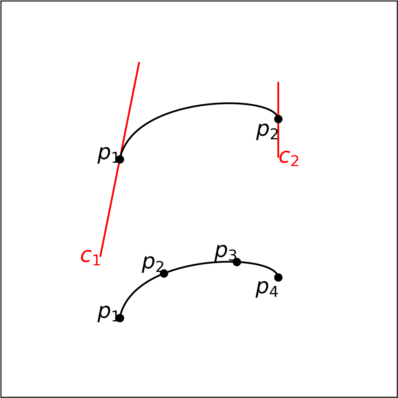
Instead, we’ll jump directly to Cubic Hermite splines. For two control points $\mathbf{p}_1$,$\mathbf{p}_2$ and two tangents $\mathbf{c}_1$, $\mathbf{c}_2$, the spline is given by⁹

$$\mathbf{Q}(t) = \begin{bmatrix} p_{1x} & c_{1x} & p_{2x} & c_{2x} \\ p_{1y} & c_{1y} & p_{2y} & c_{2y} \end{bmatrix} \cdot \begin{bmatrix} 2 & 1 & -2 & 1 \\ -3 & -2 & 3 & -1 \\ 0 & 1 & 0 & 0 \\ 1 & 0 & 0 & 0 \end{bmatrix} \cdot \begin{pmatrix} t^3 \\ t^2 \\ t \\ 1 \end{pmatrix}$$

The tangents $\mathbf{c}_1$, $\mathbf{c}_2$ correspond to the velocities at each of the positions $\mathbf{p}_1$ and $\mathbf{p}_2$. You should see a resemblence between this matrix form spline and the linear interpolation in equation $\eqref{1}$.

This composition is useful, since the server is sending player positions and velocities to the client. By substituting those for the constants in the geometry matrix $G$, we obtain a smooth curve from one position to the next.

Furthermore, since $\mathbf{G}$ and $\mathbf{B}$ don’t depend on $t$, so they can be precomputed for the interpolation steps. This is relevant for interpolating a large number of players or objects.

Figure 4: Interpolation using Cubic Hermite Splines and dead reckoning. The spline is defined by position and velocity at given points.

Figure figure 2, shows the spline interpolation in effect. It is pleasing to watch.

In networked games, player positions are sent with regular intervals. Servers run calculations at a constant rate, colloquially known as the tick rate.

For the purpose of this article, we’ll assume the server sends a message every tick – though this need not be the case for all games.

Messages from the server could contain data for the latest tick, or data for the last $n$ ticks. The client should then use the data to interpolate position and velocity, and continue with dead reckoning. Dead reckoning can be thought of as a form of prediction.

The drawback with dead reckoning is that the position may overshoot, and interpolation will move the character backwards.

To fix this, more advanced prediction models are used. These may estimating message arrival times, take into account level geometry, and incorporate inputs to improve the result. Client side movement, which can also be thought of as prediction, is often used to make a player’s controls feel snappy.

Relation to other splines

Besides Hermite splines, there are many other kinds of splines. Their main differences lie in their constraints and how the control points influence the curve.

Splines can easily be converted from one form to another by a change of basis and control points. This works as long as the degrees for the two kinds of splines match. For example, we could convert cubic Hermite splines to cubic B-splines⁸.

Recall the general matrix for for a spline shown in equation $\eqref{2}$. To convert from a basis $\mathbf{B}_1$ to another basis $\mathbf{B}_2$, we’ll use the rules for matrix inverses.

$$\begin{align*} \mathbf{Q}(t) &= \mathbf{G} \cdot \mathbf{B_1} \cdot \mathbf{T}(t)\\ &= \mathbf{G} \cdot \mathbf{B_1} \cdot (\mathbf{B}_2^{-1} \cdot \mathbf{B_2}) \cdot \mathbf{T}(t)\\ &= \mathbf{G} \cdot (\mathbf{B_1} \cdot \mathbf{B}_2^{-1}) \cdot \mathbf{B_2} \cdot \mathbf{T}(t)\\ &= \mathbf{G}_{\mathrm{new}} \cdot \mathbf{B_2} \cdot \mathbf{T}(t)\\ \end{align*}$$

Thus, we obtain the new control points $\mathbf{G}_{\mathrm{new}}$, corresponding to the new basis, by multiplying the old control points with $\mathbf{B_1} \cdot \mathbf{B}_2^{-1}$.

Splines are quite fun, so consider implementing or playing around with them. A great starting point is this interactive spline playground I found on the web.

1. We’re considering server-authoritative games here. ↩

2. Dead reckoning on Wikipedia. ↩

3. The degree of a polynomial corresponds with the highest exponent that is non-zero. The order of a polynomial is a loaded term with varying definitions. ↩

4. Advanced Engineering Mathematics, 8th Edition, ISBN 047133328-X, by Kreyzig E. ↩

5. Course notes for CS184: Foundations of Computer Graphics at UC Berkeley, 1998. ↩ ↩²

6. Course notes for CPSC 4050 / 6050 Computer Graphics at Clemson University, 2004. ↩

7. Charles Hermite on Wikipedia. ↩

8. Cubic B-Splines on Wikipedia. ↩ ↩²

9. The order of the points, control points, as well as matrices varies throughout literature. ↩